Installation
To install the latest version of OPIUM, first clone the OPIUM repository:
$ git clone https://github.com/rappegroup/opium
After navigating to the created opium directory, build the binary using:
$ ./configure
$ make all
OPIUM can now be called from the command line using:
$ ./opium input.param output.txt command1 command2 ...
To use graphical features of OPIUM, the plotting program Grace must also be installed. Grace can be downloaded from its homepage, or by running the following commands.
For Linux:
$ sudo apt-get update
$ sudo apt-get install grace
For MacOS:
$ brew install grace
Note
OPIUM is tested using Intel FORTRAN and C compilers. Although attempts have been made to allow it to be compatible with other compilers like GNU, AMD, and CRAY, there is no guarantee that outputs would align exactly.
If the above does not work, you can also try:
Downloading the statically compiled binary for OPIUM
Trying a different version of OPIUM
Using a different C or FORTRAN compiler
Help
For help, you can type into the console:
$ ./opium help
And for more specific information on command line, plotting, and keyblocks respectively:
$ ./opium -c
$ ./opium -p
$ ./opium -k
Tutorial
Using OPIUM involves setting up a parameter file and calling commands. This tutorial will illustrate that process with some very simple examples.
Hydrogen
The initial parameter file for this this Hydrogen tutorial can be
downloaded here. We will walk through how to
augment this file based on OPIUM’s outputs.
h.param:
[Atom]
H
1
100 1.00  -

[Pseudo]
1 1.80
opt

[Optinfo]
3.00  4

[XC]
gga

[Configs]
3
100 0.75 -

100 0.50 -

100 0.35 -
The [Atom] keyblock indicates that the atomic symbol is H for
hydrogen, that there is one orbital, and this orbital is “1s”,
(nlm = 100) with occupation 1.00. The - means that an eigenvalue guess
should be generated by OPIUM. The configuration specified in the [Atom] keyblock
is the reference configuration. It is used to construct the pseudopotential
and will reproduce the valence electron properties of the all-electron atom in
this configuration.
The [Pseudo] keyblock lists the number of valence orbitals, 1, and the cut-off radius
(“rc”) for the pseudopotential, which is 1.80 Angstroms here. opt indicates that
we want to use the RRKJ optimized pseudopotential method.
Since we have chosen the opt method to construct the pseudopotential, we also
need the [Optinfo] keyblock. 3.00 is the cut-off wavevector (“qc”), and
4 is the number of bessel functions to use for the pseudopotential.
The [XC] keyblock indicates what exchange-correlation (XC) functional
to use in the all-electron solve. Here we indicated gga, which means
Perdew-Burke-Ernzerhof (PBE) Generalized Gradient Approximation (GGA) will
be used.
[Configs] tests the pseudopotential on some test configurations by solving
with all-electron and solving with the pseudopotential. Here we indicate that
there are 3 tests, where we slowly remove occupation from the
“1s” occupation.
After the information has been put into a parameter file, which we will
call h.param, we can run OPIUM by calling :
$ ./opium h.param h.log ae ps nl tc rpt
This runs the following 5 commands:
ae- Perform the all-electron (AE) solve for the wavefunctionsps- Construct the pseudopotential from the AE resultsnl- Perform a non-local calculationtc- Test the effectiveness of the pseudopotential on the test configurations in[Configs]rpt- Generate a report
Running the commands should generate at least two files:
h.log- Contains all of the output from the commands and indicates any errors or warningsh.rpt- Offers a quick summary report of the pseudopotential properties
For this simple calculation, there should be no issues with that would be reflected in the log file. Then examine the pseudopotential section on the report file.
====================Optimized pseudopotential method====================

                  Pseudopotential convergence error
Orbital      [mRy/e]       [meV/e]         [mRy]        [meV]        Ghost
--------------------------------------------------------------------------
100        20.611832    280.438402     20.611832   280.438402        no

                      Tot. error =     20.611832   280.438402
This error seems very large. The pseudopotential would have approximately 280 meV error when run at a converged cut-off energy.
There are two direct ways to reduce the convergence error, by increasing rc or qc. Increasing rc leads to a less transferable potential, while increasing qc leads to a larger cut-off energy. So, lets plot the all-electron wavefunctions and see where rc is relative to to the 1s peak. This can be done by:
$ ./opium h.param h.log plot wa
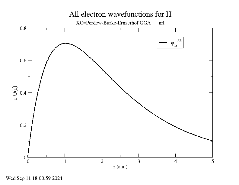
The cut-off radius is around 1.80 Angstroms and is pretty far from the peak, which
is at around 1.00 Angstroms. Therefore, it is probably better to increase qc.
Change qc from 3.0 to 4.75, so the keyblock [Optinfo] should look
like:
[Optinfo]
4.75  4
Then rerun the pseudopotential construction:
$ ./opium h.param h.log ae ps nl tc rpt
Checking the new h.rpt, the results are much better, with an error of
only 2.61 meV.
====================Optimized pseudopotential method====================

                  Pseudopotential convergence error
Orbital      [mRy/e]       [meV/e]         [mRy]        [meV]        Ghost
--------------------------------------------------------------------------
100         0.192534      2.619559      0.192534     2.619559        no

                      Tot. error =      0.192534     2.619559
Then we can check the transferability. This is a measure of how effective the
pseudopotentials is at configurations that are not the reference. Check the section for
the test configurations, and observe the lines that begin with AE-NL, which is
the difference between the all-electron and pseudopotential calculations. Since
there are 3 states in the [Configs] keyblock, there are 3 differences here:
AE-NL: Orbital Filling       Eigenvalues[mRy]         Norm[1e-3]
AE-NL- --------------------------------------------------------------
AE-NL-     100   0.750          -0.9812641227      -1.6996433434
AE-NL-   total error =           0.9812641227       1.6996433434
AE-NL: Orbital Filling       Eigenvalues[mRy]         Norm[1e-3]
AE-NL- --------------------------------------------------------------
AE-NL-     100   0.500          -3.7382161298      -3.7786023814
AE-NL-   total error =           3.7382161298       3.7786023814
AE-NL: Orbital Filling       Eigenvalues[mRy]         Norm[1e-3]
AE-NL- --------------------------------------------------------------
AE-NL-     100   0.350          -6.4826340677      -5.1011748701
AE-NL-   total error =           6.4826340677       5.1011748701
There is also a table of total energy difference:
AE-NL-   i   j         DD[mRy]        DD[meV]
AE-NL- ------------------------------------------
AE-NL-   0   1        -0.093540      -1.272673
AE-NL-   0   2        -0.639266      -8.697656
AE-NL-   0   3        -1.394842     -18.977808
AE-NL-   1   2        -0.545726      -7.424983
AE-NL-   1   3        -1.301303     -17.705135
AE-NL-   2   3        -0.755577     -10.280151
These values are good, but they could be improved. Let’s try reducing
rc from 1.80 Angstroms to 1.40 Angstroms, which is still far from
the peak. The new [Pseudo] keyblock should look like:
[Pseudo]
1 1.40
opt
We know reducing rc will increase the error as well. To compensate, we also
increase qc from 4.75 to 5.50. The new [Optinfo] keyblock is:
[Optinfo]
5.50  4
Again rerun the pseudopotential construction:
$ ./opium h.param h.log ae ps nl tc rpt
Observing h.rpt, the transferability is now much better and the error
is also within a tolerable range.
Convergence error:
====================Optimized pseudopotential method====================

                  Pseudopotential convergence error
Orbital      [mRy/e]       [meV/e]         [mRy]        [meV]        Ghost
--------------------------------------------------------------------------
100         0.422277      5.745376      0.422277     5.745376        no

                      Tot. error =      0.422277     5.745376
Transferability:
AE-NL: Orbital Filling       Eigenvalues[mRy]         Norm[1e-3]
AE-NL- --------------------------------------------------------------
AE-NL-     100   0.750          -0.3344105826      -0.7582606862
AE-NL-   total error =           0.3344105826       0.7582606862
AE-NL: Orbital Filling       Eigenvalues[mRy]         Norm[1e-3]
AE-NL- --------------------------------------------------------------
AE-NL-     100   0.500          -1.3394630445      -1.8146139118
AE-NL-   total error =           1.3394630445       1.8146139118
AE-NL: Orbital Filling       Eigenvalues[mRy]         Norm[1e-3]
AE-NL- --------------------------------------------------------------
AE-NL-     100   0.350          -2.3941203051      -2.5689934304
AE-NL-   total error =           2.3941203051       2.5689934304
AE-NL-   i   j         DD[mRy]        DD[meV]
AE-NL- ------------------------------------------
AE-NL-   0   1        -0.031401      -0.427230
AE-NL-   0   2        -0.223264      -3.037658
AE-NL-   0   3        -0.498478      -6.782148
AE-NL-   1   2        -0.191863      -2.610428
AE-NL-   1   3        -0.467078      -6.354917
AE-NL-   2   3        -0.275215      -3.744490
Since both of these are to our satisfaction, create a .upf file for
Quantum ESPRESSO by running:
$ ./opium h.param h.log all upf
Where all is a shorthand for ae ps nl tc. This should create a
h.upf file.
Further Examples
Note
Many of these walkthroughs were created with an older version of OPIUM. Results and syntax may not align exactly with newer versions.
More advanced walkthroughs are available as documents: